
- Introduction
- Fundamentals of Speech Recognition
- Dynamic Time Warping Algorithm
- Neural Network Approaches
Speech is a natural mode of communication for people. We learn all the relevant skills
during early childhood, without instruction, and we continue to rely on speech communication
throughout our lives. It comes so naturally to us that we don’t realize how complex a
phenomenon speech is. The human vocal tract and articulators are biological organs with
nonlinear properties, whose operation is not just under conscious control but also affected
by factors ranging from gender to upbringing to emotional state. As a result, vocalizations
can vary widely in terms of their accent, pronunciation, articulation, roughness, nasality,
pitch, volume, and speed; moreover, during transmission, our irregular speech patterns can
be further distorted by background noise and echoes, as well as electrical characteristics (if
telephones or other electronic equipment are used). All these sources of variability make
speech recognition, even more than speech generation, a very complex problem.
What makes people so good at recognizing speech? Intriguingly, the human brain is
known to be wired differently than a conventional computer; in fact it operates under a radically
different computational paradigm. While conventional computers use a very fast &
complex central processor with explicit program instructions and locally addressable memory,
by contrast the human brain uses a massively parallel collection of slow & simple
processing elements (neurons), densely connected by weights (synapses) whose strengths
are modified with experience, directly supporting the integration of multiple constraints, and
providing a distributed form of associative memory.
The brain’s impressive superiority at a wide range of cognitive skills, including speech
recognition, has motivated research into its novel computational paradigm since the 1940’s,
on the assumption that brainlike models may ultimately lead to brainlike performance on
many complex tasks. This fascinating research area is now known as connectionism, or the
study of artificial neural networks.
What is the current state of the art in speech recognition? This is a complex question,
because a system’s accuracy depends on the conditions under which it is evaluated: under
sufficiently narrow conditions almost any system can attain human-like accuracy, but it’s
much harder to achieve good accuracy under general conditions. The conditions of evaluation
- and hence the accuracy of any system - can vary along the following dimensions:
- Vocabulary size and confusability.
As a general rule, it is easy to discriminate
among a small set of words, but error rates naturally increase as the vocabulary
size grows. For example, the 10 digits “zero” to “nine” can be recognized essentially
perfectly , but vocabulary sizes of 200, 5000, or 100000
may have error rates of 3%, 7%, or 45%. On the other hand, even a small vocabulary can be hard to recognize if it
contains confusable words. For example, the 26 letters of the English alphabet
(treated as 26 “words”) are very difficult to discriminate because they contain so
many confusable words (most notoriously, the E-set: “B, C, D, E, G, P, T, V, Z”);
an 8% error rate is considered good for this vocabulary - Speaker dependence vs. independence.
By definition, a speaker dependent system
is intended for use by a single speaker, but a speaker independent system is
intended for use by any speaker. Speaker independence is difficult to achieve
because a system’s parameters become tuned to the speaker(s) that it was trained
on, and these parameters tend to be highly speaker-specific. - Isolated, discontinuous, or continuous speech.
Isolated speech means single
words; discontinuous speech means full sentences in which words are artificially
separated by silence; and continuous speech means naturally spoken sentences.
Isolated and discontinuous speech recognition is relatively easy because word
boundaries are detectable and the words tend to be cleanly pronounced. - Task and language constraints.
Even with a fixed vocabulary, performance will
vary with the nature of constraints on the word sequences that are allowed during
recognition. Some constraints may be task-dependent (for example, an airlinequerying
application may dismiss the hypothesis “The apple is red”); other constraints
may be semantic (rejecting “The apple is angry”), or syntactic (rejecting
“Red is apple the”). Constraints are often represented by a grammar, which ideally
filters out unreasonable sentences so that the speech recognizer evaluates only
plausible sentences. Grammars are usually rated by their perplexity, a number that
indicates the grammar’s average branching factor (i.e., the number of words that
can follow any given word). The difficulty of a task is more reliably measured by
its perplexity than by its vocabulary size. - Read vs. spontaneous speech.
Systems can be evaluated on speech that is either
read from prepared scripts, or speech that is uttered spontaneously. Spontaneous
speech is vastly more difficult, because it tends to be peppered with disfluencies
like “uh” and “um”, false starts, incomplete sentences, stuttering, coughing, and
laughter; and moreover, the vocabulary is essentially unlimited, so the system must
be able to deal intelligently with unknown words (e.g., detecting and flagging their
presence, and adding them to the vocabulary, which may require some interaction
with the user). - Adverse conditions.
A system’s performance can also be degraded by a range of
adverse conditions. These include environmental noise (e.g., noise in
a car or a factory); acoustical distortions (e.g, echoes, room acoustics); different
microphones (e.g., close-speaking, omnidirectional, or telephone); limited frequency
bandwidth (in telephone transmission); and altered speaking manner
(shouting, whining, speaking quickly, etc.).
In order to evaluate and compare different systems under well-defined conditions, a
number of standardized databases have been created with particular characteristics. For
example, one database that has been widely used is the DARPA Resource Management
database - a large vocabulary (1000 words), speaker-independent, continuous speech database,
consisting of 4000 training sentences in the domain of naval resource management,
read from a script and recorded under benign environmental conditions; testing is usually
performed using a grammar with a perplexity of 60. Under these controlled conditions,
state-of-the-art performance is about 97% word recognition accuracy (or less for simpler
systems).
Fundamentals of Speech Recognition
Speech recognition is a multileveled pattern recognition task, in which acoustical signals
are examined and structured into a hierarchy of subword units (e.g., phonemes), words,
phrases, and sentences. Each level may provide additional temporal constraints, e.g., known
word pronunciations or legal word sequences, which can compensate for errors or uncertainties
at lower levels. This hierarchy of constraints can best be exploited by combining
decisions probabilistically at all lower levels, and making discrete decisions only at the
highest level.
The structure of a standard speech recognition system is illustrated in Figure. The elements
are as follows:
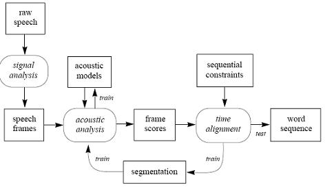
Structure of a standard speech recognition system.
- Raw speech. Speech is typically sampled at a high frequency, e.g., 16 KHz over a
microphone or 8 KHz over a telephone. This yields a sequence of amplitude values
over time. - Signal analysis. Raw speech should be initially transformed and compressed, in
order to simplify subsequent processing. Many signal analysis techniques are
available which can extract useful features and compress the data by a factor of ten
without losing any important information. Among the most popular:- Fourier analysis (FFT) yields discrete frequencies over time, which can
be interpreted visually. Frequencies are often distributed using a Mel
scale, which is linear in the low range but logarithmic in the high range,
corresponding to physiological characteristics of the human ear. - Perceptual Linear Prediction (PLP) is also physiologically motivated, but
yields coefficients that cannot be interpreted visually. - Linear Predictive Coding (LPC) yields coefficients of a linear equation
that approximate the recent history of the raw speech values. - Cepstral analysis calculates the inverse Fourier transform of the logarithm
of the power spectrum of the signal.
- Fourier analysis (FFT) yields discrete frequencies over time, which can
In practice, it makes little difference which technique is used1. Afterwards, procedures
such as Linear Discriminant Analysis (LDA) may optionally be applied to
further reduce the dimensionality of any representation, and to decorrelate the
coefficients.
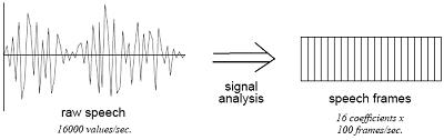
- Speech frames. The result of signal analysis is a sequence of speech frames, typically
at 10 msec intervals, with about 16 coefficients per frame. These frames may
be augmented by their own first and/or second derivatives, providing explicit
information about speech dynamics; this typically leads to improved performance.
The speech frames are used for acoustic analysis. - Acoustic models. In order to analyze the speech frames for their acoustic content,
we need a set of acoustic models. There are many kinds of acoustic models, varying
in their representation, granularity, context dependence, and other properties.
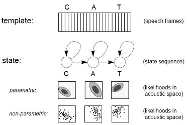
Acoustic models: template and state representations for the word “cat”.
Figure shows two popular representations for acoustic models. The simplest is
a template, which is just a stored sample of the unit of speech to be modeled, e.g.,
a recording of a word. An unknown word can be recognized by simply comparing
it against all known templates, and finding the closest match. Templates have two
major drawbacks: (1) they cannot model acoustic variabilities, except in a coarse
way by assigning multiple templates to each word; and (2) in practice they are limited
to whole-word models, because it’s hard to record or segment a sample shorter
than a word - so templates are useful only in small systems which can afford the
luxury of using whole-word models. A more flexible representation, used in larger
systems, is based on trained acoustic models, or states. In this approach, every
word is modeled by a sequence of trainable states, and each state indicates the
sounds that are likely to be heard in that segment of the word, using a probability
distribution over the acoustic space. Probability distributions can be modeled
parametrically, by assuming that they have a simple shape (e.g., a Gaussian distribution)
and then trying to find the parameters that describe it; or non-parametrically,
by representing the distribution directly (e.g., with a histogram over a
quantization of the acoustic space, or, as we shall see, with a neural network).
In this section we motivate and explain the Dynamic Time Warping algorithm, one of the
oldest and most important algorithms in speech recognition.
The simplest way to recognize an isolated word sample is to compare it against a number
of stored word templates and determine which is the “best match”. This goal is complicated
by a number of factors. First, different samples of a given word will have somewhat different
durations. This problem can be eliminated by simply normalizing the templates and the
unknown speech so that they all have an equal duration. However, another problem is that
the rate of speech may not be constant throughout the word; in other words, the optimal
alignment between a template and the speech sample may be nonlinear. Dynamic Time
Warping (DTW) is an efficient method for finding this optimal nonlinear alignment.
DTW is an instance of the general class of algorithms known as dynamic programming.
Its time and space complexity is merely linear in the duration of the speech sample and the
vocabulary size. The algorithm makes a single pass through a matrix of frame scores while
computing locally optimized segments of the global alignment path.
If
D(x,y) is the Euclidean distance between frame x of the speech sample and frame y of the
reference template, and if C(x,y) is the cumulative score along an optimal alignment path
that leads to (x,y), then
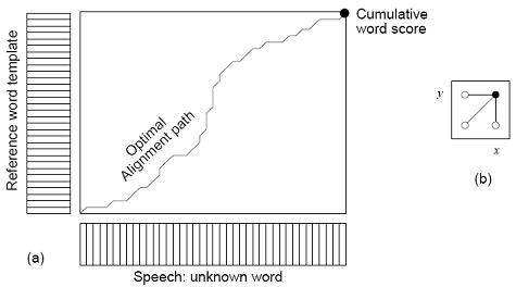
The resulting alignment path may be visualized as a low valley of Euclidean distance
scores, meandering through the hilly landscape of the matrix, beginning at (0, 0) and ending
at the final point (X, Y). By keeping track of backpointers, the full alignment path can be
recovered by tracing backwards from (X, Y). An optimal alignment path is computed for
each reference word template, and the one with the lowest cumulative score is considered to
be the best match for the unknown speech sample.
There are many variations on the DTW algorithm. For example, it is common to vary the
local path constraints, e.g., by introducing transitions with slope 1/2 or 2, or weighting the transitions in various ways, or applying other kinds of slope constraints (Sakoe and Chiba
1978). While the reference word models are usually templates, they may be state-based
models (as shown previously in Figure). When using states, vertical transitions are often
disallowed (since there are fewer states than frames), and often the goal is to maximize the
cumulative score, rather than to minimize it.
A particularly important variation of DTW is an extension from isolated to continuous
speech. This extension is called the One Stage DTW algorithm (Ney 1984). Here the goal is
to find the optimal alignment between the speech sample and the best sequence of reference
words. The complexity of the extended algorithm is still linear in the length
of the sample and the vocabulary size. The only modification to the basic DTW algorithm is
that at the beginning of each reference word model (i.e., its first frame or state), the diagonal
path is allowed to point back to the end of all reference word models in the preceding frame.
Local backpointers must specify the reference word model of the preceding point, so that
the optimal word sequence can be recovered by tracing backwards from the final point
of the word W with the best final score. Grammars can be imposed on continuous
speech recognition by restricting the allowed transitions at word boundaries.
Because speech recognition is basically a pattern recognition problem, and because neural
networks are good at pattern recognition, many early researchers naturally tried applying
neural networks to speech recognition. The earliest attempts involved highly simplified
tasks, e.g., classifying speech segments as voiced/unvoiced, or nasal/fricative/plosive. Success
in these experiments encouraged researchers to move on to phoneme classification; this
task became a proving ground for neural networks as they quickly achieved world-class
results.
There are two basic approaches to speech classification using neural networks: static and
dynamic, as illustrated in Figure.
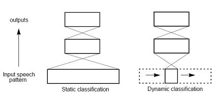
Static and dynamic approaches to classification.
In static classification, the neural network sees all of
the input speech at once, and makes a single decision. By contrast, in dynamic classification,
the neural network sees only a small window of the speech, and this window slides
over the input speech while the network makes a series of local decisions, which have to be
integrated into a global decision at a later time. Static classification works well for phoneme
recognition, but it scales poorly to the level of words or sentences; dynamic classification
scales better. Either approach may make use of recurrent connections, although recurrence
is more often found in the dynamic approach.
Phoneme classification can be performed with high accuracy by using either static or
dynamic approaches. Here we review some typical experiments using each approach.
A simple but elegant experiment was performed by Huang & Lippmann (1988), demonstrating
that neural networks can form complex decision surfaces from speech data. They
applied a multilayer perceptron with only 2 inputs, 50 hidden units, and 10 outputs, to Peterson
& Barney’s collection of vowels produced by men, women, & children, using the first
two formants of the vowels as the input speech representation. After 50,000 iterations of
training, the network produced the decision regions shown in Figure below. These decision
regions are nearly optimal, resembling the decision regions that would be drawn by hand,
and they yield classification accuracy comparable to that of more conventional algorithms,
such as k-nearest neighbor and Gaussian classification.
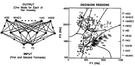
Decision regions formed by a 2-layer perceptron using backpropagation training and vowel
formant data. (From Huang & Lippmann, 1988.)
In a more complex experiment, Elman and Zipser (1987) trained a network to classify the
vowels /a,i,u/ and the consonants /b,d,g/ as they occur in the utterances ba,bi,bu; da,di,du;
and ga,gi,gu. Their network input consisted of 16 spectral coefficients over 20 frames (covering
an entire 64 msec utterance, centered by hand over the consonant’s voicing onset); this
was fed into a hidden layer with between 2 and 6 units, leading to 3 outputs for either vowel
or consonant classification. This network achieved error rates of roughly 0.5% for vowels
and 5.0% for consonants. An analysis of the hidden units showed that they tend to be feature detectors, discriminating between important classes of sounds, such as consonants versus
vowels.
Among the most difficult of classification tasks is the so-called E-set, i.e., discriminating
between the rhyming English letters “B, C, D, E, G, P, T, V, Z”. Burr (1988) applied a static
network to this task, with very good results. His network used an input window of 20 spectral
frames, automatically extracted from the whole utterance using energy information.
These inputs led directly to 9 outputs representing the E-set letters. The network was
trained and tested using 180 tokens from a single speaker. When the early portion of the
utterance was oversampled, effectively highlighting the disambiguating features, recognition
accuracy was nearly perfect.
In a seminal paper, Waibel et al (1987=1989) demonstrated excellent results for phoneme
classification using a Time Delay Neural Network (TDNN), shown in Figure.
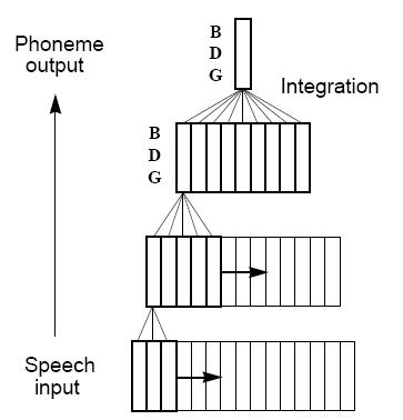
This
architecture has only 3 and 5 delays in the input and hidden layer, respectively, and the final
output is computed by integrating over 9 frames of phoneme activations in the second hidden
layer. The TDNN’s design is attractive for several reasons: its compact structure economizes
on weights and forces the network to develop general feature detectors; its hierarchy
of delays optimizes these feature detectors by increasing their scope at each layer; and its
temporal integration at the output layer makes the network shift invariant (i.e., insensitive to
the exact positioning of the speech). The TDNN was trained and tested on 2000 samples of /
b,d,g/ phonemes manually excised from a database of 5260 Japanese words. The TDNN
achieved an error rate of 1.5%, compared to 6.5% achieved by a simple HMM-based recognizer.