• Introduction
• Neocognitron Architecture
• Neocognitron data processing
• Training Weights on the S-Layers

Introduction

Artificial neural network architectures such as backpropagation tend to have general applicability. We can use a single network type in many different applications by changing the network’s size, parameters, and training sets. In contrast, the developers of the neocognitron set out to tailor architecture for a specific application: recognition of handwritten characters. Such a system has a great deal of practical application, although, judging from the introductions to some of their papers, Fukushima and his coworkers appear to be more interested in developing a model of the brain .To that end, their design was based on the seminal work performed by Hubel and Weisel elucidating some of the functional architecture of the visual cortex.

We could not begin to provide a complete accounting of what is knownabout the anatomy and physiology of the mammalian visual system. Nevertheless, we shall present a brief and highly simplified description of some of that system’s features as an aid to understanding thejbasis of the neocognitron design.

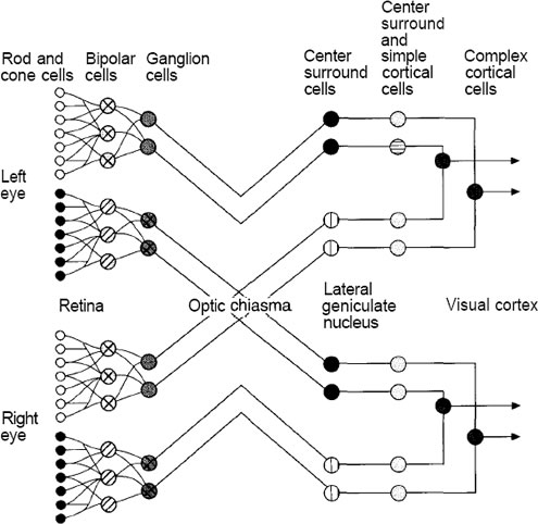
Figure A: Visual pathways from the eye to the primary visual cortex
are shown. Some nerve fibers from each eye cross over into
the opposite hemisphere of the brain, where they meet nerve
fibers from the other eye at the LGN. From the LGN, neurons
project back to area 17. From area 17, neurons project into
other cortical areas, other areas deep in the brain, and also
back to the LGN.
Figure shows the main pathways for neurons leading from the retina back to the area of the brain known as the viiual, or striate, cortex. This area is also known as area 17. The optic nerve ii made up of axons from nerve cells called retinal ganglia. The ganglia receive stimulation indirectly from the light-receptive rods and cones through several intervening neurons. Hubel and Weisel used an amazing technique to discern the function of the various nerve cells in the visual system. They used microelectrodes to record the response of individual neurons in the cortex while stimulating the retina with light. By applying a variety of patterns and shapes, they were able to determine the particular stimulus to which a neuron was most sensitive.

The retinal ganglia and the cells of the lateral geniculate nucleus (LGN) appear to have circular receptive fields.

They respond most strongly to circular spots of light of a particular size on a particular part of the retina. The part of the retina responsible for stimulating a particular ganglion cell is called the receptive field of the ganglion. Some of these receptive fields give an excitatory response to a centrally located spot of light, and an inhibitory response to a larger, more diffuse spot of light. These fields have an on-center off-surround response characteristic. Other receptive fields have the opposite characteristic, with an inhibitory response to the centrally located spot—an off-center on-surround response characteristic.

The visual cortex itself is composed of six layers of neurons. Most of the neurons from the LGN terminate on cells in layer IV. These cells have circularly symmetric receptive fields like the retinal ganglia and the cells of the LGN. Further along the pathway, the response characteristic of the cells begins to increase in complexity. Cells in layer IV project to a group of cells directly above called simple cells. Simple cells respond to line segments having a particular orientation. Simple cells project to cells called complex cells. Complex cells respond to lines having the same orientation as their corresponding simple cells, although complex cells appear to integrate their response over a wider receptive field. In other words, complex cells are less sensitive to the position of the line on the retina than are the simple cells. Some complex cells are sensitive to line segments of a particular orientation that are moving in a particular direction.

Cells in different layers of area 17 project to different locations of the brain. For example, cells in layers II and III project to cells in areas 18 and 19. These areas contain cells called hypercomplex cells. Hypercomplex cells respond to lines that form angles or corners and that move in various directions across the receptive field.

The picture that emerges from these studies is that of a hierarchy of cells with increasingly complex response characteristics. It is not difficult to extrapolate this idea of a hierarchy into one where further data abstraction takes place at higher and higher levels. The neocognitron design adopts this hierarchical structure in a layered architecture, as illustrated schematically in Figure
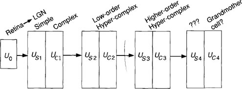Figure B: The neocognitron hierarchical structure is shown. Each box
represents a level in the neocognitron comprising a simplecell
layer, usi, and a complex-cell layer, Ua, where i is
the layer number. U0 represents signals originating on the
retina. There is also a suggested mapping to the hierarchical
structure of the brain. The network concludes with single
cells that respond to complex visual stimuli. These final cells
are often called grandmother cells after the notion that there
may be some cell in your brain that responds to complex
visual stimuli, such as a picture of your grandmother.

We remind you that the description of the visual system that we have presented
here is highly simplified. There is a great deal of detail that we have
omitted. The visual system does not adhere to a strict hierarchical structure
as presented here. Moreover, we do not subscribe to the notion that grandmother
cells per se exist in the brain. We know from experience that strict
adherence to biology often leads to a failed attempt to design a system to perform
the same function as the biological prototype: Flight is probably the most
significant example. Nevertheless, we do promote the use of neurobiological
results if they prove to be appropriate. The neocognitron is an excellent example
of how neurobiological results can be used to develop a new network
architecture.

NEOCOGNITRON ARCHITECTURE

The neocognitron design evolved from an earlier model called the cognitron,
and there are several versions of the neocognitron itself. The one that we shall
describe has nine layers of PEs (Processing elements), including the retina layer. The system was
designed to recognize the numerals 0 through 9, regardless of where they are
placed in the field of view of the retina. Moreover, the network has a high degree
of tolerance to distortion of the character and is fairly insensitive to the size of
the character. This first architecture contains only feedforward connections.

The PEs of the neocognitron are organized into modules that we shall refer to
as levels. A single level is shown in Figure 10.3. Each level consists of two
layers: a layer of simple cells, or S-cells, followed by a layer of complex
cells, or C-cells. Each layer, in turn, is divided into a number of planes,
each of which consists of a rectangular array of PEs. On a given level, the
S-layer and the C-layer may or may not have the same number of planes.
All planes on a given layer will have the same number of PEs; however, the
number of PEs on the S-planes can be different from the number of PEs on
the C-planes at the same level. Moreover, the number of PEs per plane can
vary from level to level. There are also PEs called Vs-cells and Vc-cells that
are not shown in the figure. These elements play an important role in the
processing, but we can describe the functionality of the system without reference
to them.

We construct a complete network by combining an input layer, which we
shall call the retina, with a number of levels in a hierarchical fashion, as shown
in Figure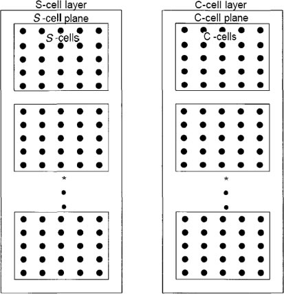

Figure C: A single level of a neocognitron is shown. Each level consists
of two layers, and each layer consists of a number of planes.
The planes contain the PEs in a rectangular array. Data pass
from the S-layer to the C-layer through connections that are
not shown here. In neocognitrons having feedback, there also
will be connections from the C-layer to the S-layer.

That figure shows the number of planes on each layer for the
particular implementation that we shall describe here. We call attention to the fact that there is nothing, in principle, that dictates a limit to the size of the
network in terms of the number of levels.
The interconnection strategy is unlike that of networks that are fully interconnected
between layers, such as the backpropagation network.

Figure D shows a schematic illustration of the way units are
connected in the neocognitron.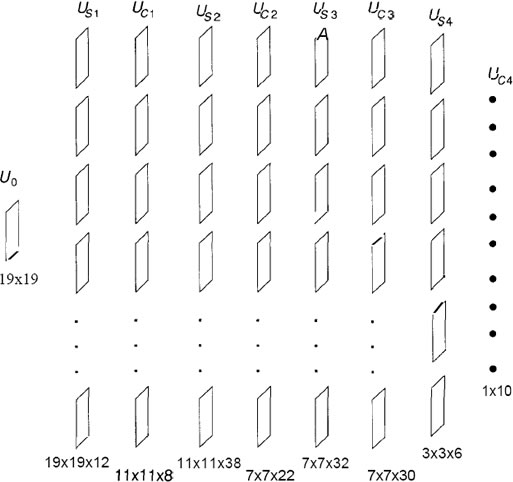

The figure D shows the basic organization of the neocognitron
for the numeral-recognition problem. There are nine layers,
each with a varying number of planes. The size of each layer,
in terms of the number of processing elements, is given below
each layer. For example, layer Uc2 has 22 planes of 7 x 7
processing elements arranged in a square matrix. The layer
of C-cells on the final level is made up of 10 planes, each
of which has a single element. Each element corresponds to
one of the numerals from 0 to 9. The identification of the
pattern appearing on the retina is made according to which
C-cell on the final level has the strongest response.

As we look deeper into the network, the S-cells respond to features at higher
levels of abstraction; for example, corners with intersecting lines at various angles and orientations. The C-cells integrate the responses of groups of Scells.
Because each S-cell is looking for the same feature in a different location,
the C-cells’ response is less sensitive to the exact location of the feature on the
input layer. This behavior is what gives the neocognitron its ability to identify
characters regardless of their exact position in the field of the retina. By the
time we have reached the final layer of C-cells, the effective receptive field of each cell is the entire retina. Figure 10.6 shows the character identification
process schematically.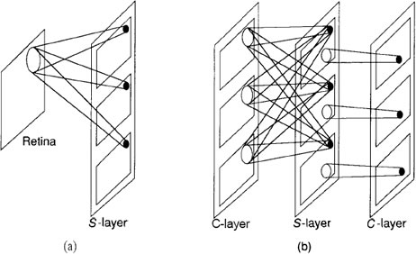

Figure F: This diagram is a schematic representation of the
interconnection strategy of the neocognitron. (a) On the first
level, each S unit receives input connections from a small
region of the retina. Units in corresponding positions on all
planes receive input connections from the same region of
the retina. The region from which an S-cell receives input
connections defines the receptive field of the cell, (b) On
intermediate levels, each unit on an s-plane receives input
connections from corresponding locations on all C-planes in
the previous level. C-eelIs have connections from a region of
S-cells on the S level preceding it. If the number of C-planes
is the same as that of S-planes at that level, then each C-cell
has connections from S-cells on a single s-plane. If there
are fewer C-planes than S-planes, some C-cells may receive
connections from more than one S-plane.

Each cell in a plane on the first S-layer receives inputs from
a single input layer-namely, the retina. On subsequent layers, each S-cell
plane receives inputs from each of the C-cell planes immediately preceding
it. The situation is slightly different for the C-cell planes. Typically, each
cell on a C-cell plane examines a small region of S-cells on a single S-cell
plane. For example, the first C-cell plane on layer 2 would have connections
to only a region of S-cells on the first S-cell plane of the previous layer. Reference back to Figure D reveals that there is not necessarily a one-to-one
correspondence between C-cell planes and S-cell planes at each layer in the
system. This discrepancy occurs because the system designers found it advantageous
to combine the inputs from some S-planes to a single C-plane if the
features that the S-planes were detecting were similar. This tuning process
is evident in several areas of the network architecture and processing equations.

Figure G: This figure illustrates how the neocognitron performs
its character-recognition function. The neocognitron
decomposes the input pattern into elemental parts consisting
of line segments at various angles of rotation. The system
then integrates these elements into higher-order structures at
each successive level in the network. Cells in each level
integrate the responses of cells in the previous level over a
finite area. This behavior gives the neocognitron its ability to
identify characters regardless of their exact position or size
in the field of view of the retina. Source: Reprinted with
permission from Kunihiko Fukushima, “A neural network for
visual pattern recognition.” IEEE Computer, March 1988. ©
1988 IEEE.

The weights on connections to S-cells are determined by a training process. Unlike in many other network architectures
(such as backpropagation), where each unit has a different weight vector,
all S-cells on a single plane share the same weight vector. Sharing weights
in this manner means that all S-cells on a given plane respond to the identical
feature in their receptive fields, as we indicated. Moreover, we need to train only one S-cell on each plane, then to distribute the resulting weights to the
other cells.
The weights on connections to C-cells are not modifiable in the sense that
they are not determined by a training process. All C-cell weights are usually
determined by being tailored to the specific network architecture. As with Splanes,
all cells on a single C-plane share the same weights. Moreover, in some
implementations, all C-planes on a given layer share the same weights.

NEOCOGNITRON DATA PROCESSING

In this section we shall discuss the various processing algorithms of the neocognitron
cells. First we shall look at the S-cell data processing including the
method used to train the network. Then, we shall describe processing on the
C-layer.

S-Cell Processing

We shall first concentrate on the cells in a single plane of Js, as indicated in
Figure H

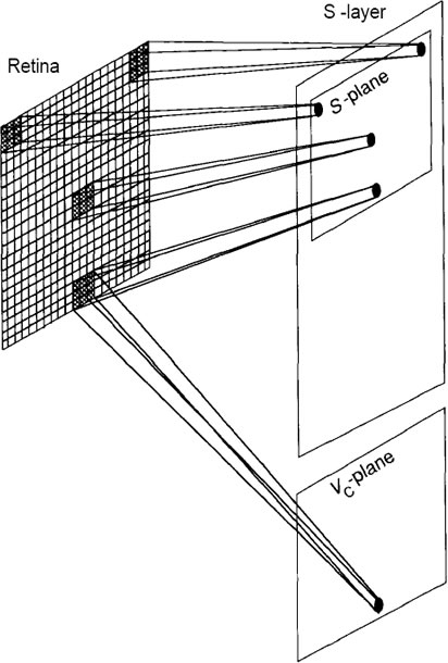
Figure H: The retina, layer U0, is a 19-by-19-pixel array, surrounded by
inactive pixels to account for edge effects as described in the
text. One of the S-planes is shown, along with an indication
of the regions of the retina scanned by the individual cells.
Associated with each S-layer in the system is a plane of vrcells.
These cells receive input connections from the same
receptive field as do the S-cells in corresponding locations in
the plane. The processing done by these Vc-cells is described
in the text.
We shall assume that the retina, layer Uo, is an array of 19 by 19
pixels. Therefore, each Usi plane will have an array of 19 by 19 cells. Each
plane scans the entire retina for a particular feature. As indicated in the figure,
each cell on a plane is looking for the identical feature but in a different location
on the retina. Each S-cell receives input connections from an array of 3 by 3
pixels on the retina. The receptive field of each S-cell corresponds to the 3 by 3
array centered on the pixel that corresponds to the cell’s location on the plane.
When building or simulating this network, we must make allowances for
edge effects. If we surround the active retina with inactive pixels (outputs always
set to zero), then we can automatically account for cells whose fields
of view are centered on edge pixels. Neighboring S-cells scan the retina array
displaced by one pixel from each otlier. In this manner, the entire image
is scanned from left to right and top to bottom by the cells in each Splane.

A
single plane of Vc-cells is associated with the S-layer, as indicated in
Figure H. The Vc-plane contains the same number of cells as does each Splane.
Vc-cells have the same receptive fields as the S-cells in corresponding
locations in the plane. The output of a Vc-cell goes to a single S-cell in every
plane in the layer. The S-cells that receive inputs from a particular Vc-cell
are those that occupy a position in the plane corresponding to the position of
the Vc-cell. The output of the Vc-cell has an inhibitory effect on the S-cells.
Figure I shows the details of a single S-cell along with its corresponding
inhibitory cell.


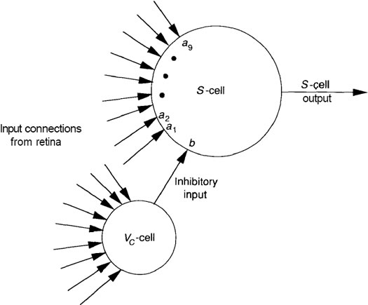
FIGURE I: A single 5-cell and corresponding inhibitory cell on the Us
layer are shown. Each unit receives the identical nine inputs
from the retina layer. The weights, a,, on the S-ce\ determine
the feature for which the cell is sensitive. Both the a, weights
on connections from the retina, and the weight, b, from the
Vr-cells are modifiable and are determined during a training
process, as described in the text.

Up to now, we have been discussing the first S-layer, in which cells receive
input connections from a single plane (in this case the retina) in the previous
layer. For what follows, we shall generalize our discussion to include the case of layers deeper in the network where an S-cell will receive input connections
from all the planes on the previous C-layer.
Let the index k refer to the kth plane on level 1. We can label each cell
on a plane with a two-dimensional vector, with n indicating its position on the
plane; then, we let the vector v refer to the relative position of a cell in the
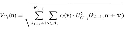
previous layer lying in the receptive field of unit n. With these definitions, we can write the following equation for the output of any 5-cell:


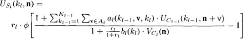
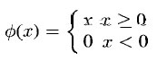
where the function Φ is a linear threshold function given by

Let’s dissect these equations in some detail. The inner summation of
first equation is the usual sum-of-products calculation of inputs, UCi-1(ki-1,n+v),
and weights, ai(ki-1, v. ki). The sum extends over all units in the previous Clayer
that lie within the receptive field of unit n. Those units are designated
by the vector n + v. Because we shall assume that all weights and cell output
values are nonnegative, the sum-of-products calculation yields a measure of how
closely the input pattern matches the weight vector on a unit.2 We have labeled
the receptive field Ai, indicating that the geometry of the receptive field is the
same for all units on a particular layer. The outer summation of the equation
extends over all of the ki-1planes of the previous C-layer. In the case of Us1 ,
there would be no need for this outer summation.

The product, bi(ki) . Vc,(n), in the denominator of Equation, represents the
inhibitory contribution of the Vc-cell. The parameter ri, where 0 < ri < ∞, determines the cell's selectivity for a specific pattern. The factor ri/(1 + ri)
goes from zero to one as ri goes from zero to infinity. Thus, for small values
of r;, the denominator of Equation could be relatively small compared to the
numerator even if the input pattern did not exactly match the weight vector. This
situation could result in a positive argument to the Φ function. If ri were large,
then the match between the input pattern and the weights in the numerator of
the equation would have to be more exact to overcome the inhibitory effects of the
Vc-cell input. Notice also that this same ri parameter appears as a multiplicative
factor of the 0 function. If ri is small, and cell selectivity is small, this factor
ensures that the output from the cell itself cannot become very large.
We can view the function of r; in another way. We rewrite the argument
of the function in the equation as


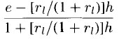
where e is the net excitatory term and h is the net inhibitory term. According
to function , the S-cell output will be nonzero only if

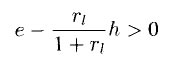
or

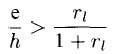
Thus, the quantity ri determines the minimum relative strength of excitation
versus inhibition that will result in a nonzero output of the unit. As r; increases,
ri/(l + ri) → 1. Therefore, a larger ri requires a larger excitation relative to
inhibition for a nonzero output.

Notice that neither of the weight expressions, ai(ki-1,v,ki), or bi(ki) depend
explicitly on the position, n, of the cell. Remember that all cells on a
plane share the same weights, even the bi(ki) weights, which we did not discuss
previously.
We must now specify the output from the inhibitory nodes. The Vc-cell at
position n has an output value of

where ci(v) is the weight on the connection from a cell at position v of the
Vc -cell’s receptive field. These weights are not subject to training. They can
take the form of any normalized function that decreases monotonically as the
magnitude of v increases.

Training Weights on the S-Layers

In principle, training proceeds as it does for many
networks. First, an input pattern is presented at the input layer and the data are
propagated through the network. Then, weights are allowed to make incremental
adjustments according to the specified algorithm. After weight updates have
occurred, a new pattern is presented at the input layer, and the process is repeated
with all patterns in the training set until the network is classifying the input
patterns properly.
In the neocognitron, sharing of weights on a given plane means that only a
single cell on each plane needs to participate in the learning process. Once its
weights have been updated, a copy of the new weight vector can be distributed
to the other cells on the same plane. To understand how this works, we can
think of the 5-planes on a given layer as being stacked vertically on top of one
another, aligned so that cells at corresponding locations are directly on top of one
another. We can now imagine many overlapping columns running perpendicular
to this stack. These columns define groups of S-cells, where all of the members
in a group have receptive fields in approximately the same location of the input
layer.

Unsupervised training:With this model in mind, we now apply an input pattern and examine
the response of the S’-cells in each column. To ensure that each 5-cell provides
a distinct response, we can initialize the a; weights to small, positive
random values. The bi weights on the inhibitory connections can be initialized
to zero. We first note the plane and position of the S-cell whose response is
the strongest in each column. Then we examine the individual planes so that,
if one plane contains two or more of these S-cells, we disregard all but the
cell responding the strongest. In this manner, we will locate the S-cell on each
plane whose response is the strongest, subject to the condition that each of those
cells is in a different column. Those S-cells become the prototypes, or representatives,
of all the cells on their respective planes. Likewise, the strongest
responding Vf-cell is chosen as the representative for the other cells on the
Vc-plane.
Once the representatives are chosen, weight updates are made according to
the following equations:

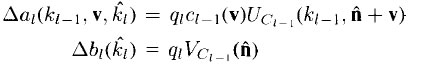
where qi is the learning rate parameter, ci-1(v), is the monotonically decreasing
function as described in the previous section, and the location of the representative
for plane ki is A.
Notice that the largest increases in the weights occur on those connections
that have the largest input signal, Uci-1(ki-1, n + v). Because the 5-cell whose
weights are being modified was the one with the largest output, this learning
algorithm implements a form of Hebbian learning. Notice also that weights can
only increase, and that there is no upper bound on the weight value. Once the cells on a given plane begin to respond to a certain feature, they
tend to respond less to other features. lfter a short time, each plane will have
developed a strong response to a particular feature. Moreover, as we look deeper
into the network, planes will be responding to more complex features.

Other Learning Methods. The designers of the original neocognitron knew
to what features they wanted each level, and each plane on a level, to respond.
Under these circumstances, a set of training vectors can be developed for each
layer, and the layers can be trained independently.
It is also possible to select the representative cell for each plane in advance.
Care must be taken, however, to ensure that the input pattern is presented in the
proper location with respect to the representative’s receptive field. Here again,
some foreknowledge of the desired features is required.