Home | Blog | Site Map | Link Directory | References |

Intelligent Search

Problem Solving

• Introduction
• General Problem Solving Approaches
  • Breadth First Search
  • Depth First Search
  • Iterative Deepening Search
  • Hill Climbing
  • Simulated Annealing
• Heuristic Search
  • Heuristic Search for OR Graphs

Introduction

Problem solving requires two prime considerations: first representation of the problem by an appropriately organized state space and then testing the existence of a well-defined goal state in that space. Identification of the goal state and determination of the optimal path, leading to the goal through one or more transitions from a given starting state, will be addressed in this chapter in sufficient details. The chapter, thus, starts with some well-known search algorithms, such as the depth first and the breadth first search, with special emphasis on their results of time and space complexity. It then gradually explores the 'heuristic search' algorithms, where the order of visiting the states in a search space is supported by thumb rules, called heuristics, and demonstrates their applications in complex problem solving. It also discusses some intelligent search algorithms for game playing.

Common experience reveals that a search problem is associated with two important issues: first 'what to search' and secondly 'where to search'. The first one is generally referred to as 'the key', while the second one is termed 'search space'. In AI the search space is generally referred to as a collection of states and is thus called state space. Unlike common search space, the state space in most of the problems in AI is not completely known, prior to solving the problem. So, solving a problem in AI calls for two phases: the generation of the space of states and the searching of the desired problem state in that space. Further, since the whole state space for a problem is quite large, generation of the whole space prior to search may cause a significant blockage of storage, leaving a little for the search part. To overcome this problem, the state space is expanded in steps and the desired state, called "the goal", is searched after each incremental expansion of the state space.

Depending on the methodology of expansion of the state space and consequently the order of visiting the states, search problems are differently named in AI. For example, consider the state space of a problem that takes the form of a tree. Now, if we search the goal along each breadth of the tree, starting from the root and continuing up to the largest depth, we call it breadth first search. On the other hand, we may sometimes search the goal along the largest depth of the tree, and move up only when further traversal along the depth is not possible. We then attempt to find alternative offspring of the parent of the node (state) last visited. If we visit the nodes of a tree using the above principles to search the goal, the traversal made is called depth first traversal and consequently the search strategy is called depth first search. We will shortly explore the above schemes of traversal in a search space. One important issue, however, needs mention at this stage. We may note that the order of traversal and hence search by breadth first or depth first manner is generally fixed by their algorithms. Thus once the search space, here the tree, is given, we know the order of traversal in the tree. Such types of traversal are generally called 'deterministic'. On the other hand, there exists an alternative type of search, where we cannot definitely say which node will be traversed next without computing the details in the algorithm. Further, we may have transition to one of many possible states with equal likelihood at an instance of the execution of the search algorithm. Such a type of search, where the order of traversal in the tree is not definite, is generally termed 'nondeterministic'. Most of the search problems in AI are non-deterministic.

General Problem Solving Approaches

There exist quite a large number of problem solving techniques in AI that rely on search. The simplest among them is the generate and test method. The algorithm for the generate and test method can be formally stated as follows:

It is clear from the above algorithm that the algorithm continues the possibility of exploring a new state in each iteration of the repeat-until loop and exits only when the current state is equal to the goal. Most important part in the algorithm is to generate a new state. This is not an easy task. If generation of new states is not feasible, the algorithm should be terminated. In our simple algorithm, we, however, did not include this intentionally to keep it simplified.

But how does one generate the states of a problem? To formalize this, we define a four tuple, called state space, denoted by
{ nodes, arc, goal, current },
where nodes represent the set of existing states in the search space; an arc denotes an operator applied to an existing state to cause transition to another state; goal denotes the desired state to be identified in the nodes; and current represents the state, now generated for matching with the goal.

We will now present two typical algorithms for generating the state
space for search. These are depth first search and breadth first search.

Breadth First Search

The breadth first search algorithm visits the nodes of the tree along its
breadth, starting from the level with depth 0 to the maximum depth. It can be
easily realized with a queue. For instance, consider the tree, given in figure.
Here, the nodes in the tree are traversed following their ascending ordered labels.

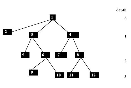
The order of traversal in a tree of depth 3 by breadth first manner.

The algorithm for traversal in a tree by depth first manner can be presented with a queue as follows:

The breadth first search algorithm, presented above, rests on a simple principle. If the current node is not the goal add the offspring of the current in any order to the rear end of the queue and redefine the front element of the queue as the current. The algorithm terminates, when the goal is found.

First few steps of breadth first search on the tree of fig.

Time Complexity
For the sake of analysis, we consider a tree of equal branching factor from each node = b and largest depth = d. Since the goal is not located within depth (d-1), the number of false search is given by

Further, the first state within the fringe nodes could be the goal. On the other hand, the goal could be the last visited node in the tree. Thus, on an average, the number of fringe nodes visited is given by

Consequently, the total number of nodes visited in an average case becomes

Since the time complexity is proportional to the number of nodes visited, therefore, the above expression gives a measure of time complexity.

Space Complexity
The maximum number of nodes will be placed in the queue, when the leftmost node at depth d is inspected for comparison with the goal. The queue length under this case becomes bd. The space complexity of the algorithm that depends on the queue length, in the worst case, thus, is of the order of bd. In order to reduce the space requirement, the generate and test algorithm is realized in an alternative manner, as presented below.

Depth First Search

The depth first search generates nodes and compares them with the goal along the largest depth of the tree and moves up to the parent of the last visited node, only when no further node can be generated below the last visited node. After moving up to the parent, the algorithm attempts to generate a new offspring of the parent node. The above principle is employed recursively to each node of a tree in a depth first search. One simple way to realize the recursion in the depth first search algorithm is to employ a stack. A stackbased realization of the depth first search algorithm is presented below.

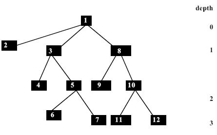
Fig. A:Depth first search on a tree, where the node numbers denote the order of visiting that node.

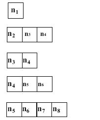
In the above algorithm, a starting node is placed in the stack, the top of which is pointed to by the stack-top. For examining the node, it is popped out from the stack. If it is the goal, the algorithm terminates, else its children are pushed into the stack in any order. The process is continued until the stack is empty. The ascending order of nodes in fig. A represents its traversal on the tree by depth first manner. The contents of the stack at the first few iterations are illustrated below in fig. B. The arrowhead in the figure denotes the position of the stack-top.

Fig. B: A snapshot of the stack at the first few iterations.

Space Complexity
Maximum memory in depth first search is required, when we reach the largest depth at the first time. Assuming that each node has a branching factor b, when a node at depth d is examined, the number of nodes saved in memory are all the unexpanded nodes up to depth d plus the node being examined. Since at each level there are (b-1) unexpanded nodes, the total number of memory required = d (b -1) +1. Thus the space complexity of depth first search is a linear function of b, unlike breadth first search, where it is an exponential function of b. This, in fact, is the most useful aspect of the depth first search.

Time Complexity
If we find the goal at the leftmost position at depth d, then the number of nodes examined = (d +1). On the other hand, if we find the goal at the extreme right at depth d, then the number of nodes examined include all the nodes in the tree, which is

So, the total number of nodes examined in an average case

This is the average case time complexity of the depth first search algorithm. Since for large depth d, the depth first search requires quite a large runtime, an alternative way to solve the problem is by controlling the depth of the search tree. Such an algorithm, where the user mentions the initial depth cut-off at each iteration, is called an Iterative Deepening Depth First Search or simply an Iterative deepening search.

Iterative Deepening Search

When the initial depth cut-off is one, it generates only the root node and examines it. If the root node is not the goal, then depth cut-off is set to two and the tree up to depth 2 is generated using typical depth first search. Similarly, when the depth cut-off is set to m, the tree is constructed up to depth m by depth first search. One may thus wonder that in an iterative deepening search, one has to regenerate all the nodes excluding the fringe nodes at the current depth cut-off. Since the number of nodes generated by depth first search up to depth h is

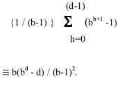
the total number of nodes expanded in failing searches by an iterative deepening search will be

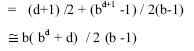
The last pass in the algorithm results in a successful node at depth d, the average time complexity of which by typical depth first search is given by

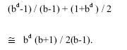
Thus the total average time complexity is given by

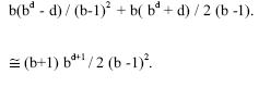
Consequently, the ratio of average time complexity of the iterative deepening search to depth first search is given by

The iterative deepening search thus does not take much extra time, when compared to the typical depth first search. The unnecessary expansion of the entire tree by depth first search, thus, can be avoided by iterative deepening. A formal algorithm of iterative deepening is presented below.

The breadth first, depth first and the iterative deepening search can be equally used for Generate and Test type algorithms. However, while the breadth first search requires an exponential amount of memory, the depth first search calls for memory proportional to the largest depth of the tree. The iterative deepening, on the other hand, has the advantage of searching in a depth first manner in an environment of controlled depth of the tree.

Hill Climbing

The 'generate and test' type of search algorithms presented above only expands the search space and examines the existence of the goal in that space. An alternative approach to solve the search problems is to employ a function f(x) that would give an estimate of the measure of distance of the goal from node x. After f(x) is evaluated at the possible initial nodes x, the nodes are sorted in ascending order of their functional values and pushed into a stack in the ascending order of their 'f' values. So, the stack-top element has the least f value. It is now popped out and compared with the goal. If the stack-top element is not the goal, then it is expanded and f is measured for each of its children. They are now sorted according to their ascending order of the functional values and then pushed into the stack. If the stack-top element is the goal, the algorithm exits; otherwise the process is continued until the stack becomes empty. Pushing the sorted nodes into the stack adds a depth first flavor to the present algorithm. The hill climbing algorithm is formally presented below.

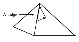
Moving along a ridge in two steps (by two successive operators) in hill climbing.

The hill climbing algorithm too is not free from shortcomings. One common problem is trapping at local maxima at a foothill. When trapped at local maxima, the measure of f at all possible next legal states yield less promising values than the current state. A second drawback of the hill climbing is reaching a plateau. Once a state on a plateau is reached, all legal next states will also lie on this surface, making the search ineffective. A new algorithm, called simulated annealing, discussed below could easily solve the first two problems. Besides the above, another problem that too gives us trouble is the traversal along the ridge. A ridge (vide figure above) on many occasions leads to a local maxima. However, moving along the ridge is not possible by a single step due to non-availability of appropriate operators. A multiple step of movement is required to solve this problem.

Simulated Annealing

"Annealing" is a process of metal casting, where the metal is first melted at a high temperature beyond its melting point and then is allowed to cool down, until it returns to the solid form. Thus in the physical process of annealing, the hot material gradually loses energy and finally at one point of time reaches a state of minimum energy. A common observation reveals that most physical processes have transitions from higher to lower energy states, but there still remains a small probability that it may cross the valley of energy states [2] and move up to a energy state, higher than the energy state of the valley. The concept can be verified with a rolling ball. For instance, consider a rolling ball that falls from a higher (potential) energy state to a valley and then moves up to a little higher energy state (vide figure below). The probability of such

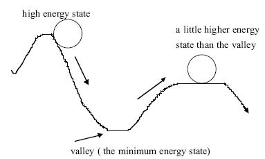
A rolling ball passes through a valley to a higher energy state.
transition to a higher energy state, however, is very small and is given by

where p is the probability of transition from a lower to a higher energy state, ΔE denotes a positive change in energy, K is the Boltzman constant and T is the temperature at the current thermal state. For small ΔE, p is higher than the value of p, for large ΔE. This follows intuitively, as w.r.t the example of ball movement, the probability of transition to a slightly higher state is more than the probability of transition to a very high state. An obvious question naturally arises: how to realize annealing in search? Readers, at this stage, would remember that the need for simulated annealing is to identify the direction of search, when the function f yields no better next states than the current state. Under this circumstance, ΔE is computed for all possible legal next states and p' is also evaluated for each such next state by the following formula:

A random number in the closed interval of [0,1] is then computed and p' is compared with the value of the random number. If p' is more, then it is selected for the next transition. The parameter T, also called temperature, is gradually decreased in the search program. The logic behind this is that as T decreases, p' too decreases, thereby allowing the algorithm to terminate at a stable state. The algorithm for simulated annealing is formally presented below.

The algorithm is similar to hill climbing, if there always exists at least one better next state than the state, pointed to by the stack-top. If it fails, then the last begin-end bracketed part of the algorithm is invoked. This part corresponds to simulated annealing. It examines each legal next state one by one, whether the probability of occurrence of the state is higher than the random value in [0,1]. If the answer is yes, the state is selected, else the next possible state is examined. Hopefully, at least one state will be found whose probability of occurrence is larger than the randomly generated probability.

Another important point that we did not include in the algorithm is the process of computation of ΔE. It is computed by taking the difference of the value of f of the next state and that of the current (stack-top) state.

The third point to note is that T should be decreased once a new state with less promising value is selected. T is always kept non-negative. When T becomes zero, p' will be zero and thus the probability of transition to any other state will be zero.

Heuristic Search

This section is devoted to solve the search problem by a new technique, called heuristic search. The term "heuristics" stands for " thumb rules", i.e., rules which work successfully in many cases but its success is not guaranteed.

In fact, we would expand nodes by judiciously selecting the more promising nodes, where these nodes are identified by measuring their strength compared to their competitive counterparts with the help of specialized intuitive functions, called heuristic functions.

Heuristic search is generally employed for two distinct types of problems:
i) forward reasoning and
ii) backward reasoning.
We have already discussed that in a forward reasoning problem we move towards the goal state from a pre-defined starting state, while in a backward reasoning problem, we move towards the starting state from the given goal. The former class of search algorithms, when realized with heuristic functions, is generally called heuristic Search for OR-graphs or the Best First search Algorithms. It may be noted that the best first search is a class of algorithms, and depending on the variation of the performance measuring function it is differently named. One typical member of this class is the algorithm A*. On the other hand, the heuristic backward reasoning algorithms are generally called AND-OR graph search algorithms and one ideal member of this class of algorithms is the AO* algorithm. We will start this section with the best first search algorithm.

Heuristic Search for OR Graphs

Most of the forward reasoning problems can be represented by an OR-graph, where a node in the graph denotes a problem state and an arc represents an application of a rule to a current state to cause transition of states. When a number of rules are applicable to a current state, we could select a better state among the children as the next state. We remember that in hill climbing, we ordered the promising initial states in a sequence and examined the state occupying the beginning of the list. If it was a goal, the algorithm was terminated. But, if it was not the goal, it was replaced by its offsprings in any order at the beginning of the list. The hill climbing algorithm thus is not free from depth first flavor. In the best first search algorithm to be devised shortly, we start with a promising state and generate all its offsprings. The performance (fitness) of each of the nodes is then examined and the most promising node, based on its fitness, is selected for expansion. The most promising node is then expanded and the fitness of all the newborn children is measured. Now, instead of selecting only from the generated children, all the nodes having no children are examined and the most promising of these fringe nodes is selected for expansion. Thus unlike hill climbing, the best first search provides a scope of corrections, in case a wrong step has been selected earlier. This is the prime advantage of the best first search algorithm over hill climbing. The best first search algorithm is formally presented below.

As already pointed out, the best first search algorithm is a generic algorithm and requires many more extra features for its efficient realization. For instance, how we can define f is not explicitly mentioned in the algorithm. Further, what happens if an offspring of the current node is not a fringe node. The A* algorithm to be discussed shortly is a complete realization of the best first algorithm that takes into account these issues in detail. The following definitions, however, are required for presenting the A* algorithm. These are in order.

Definition: A node is called open if the node has been generated and the h' (x) has been applied over it but it has not been expanded yet.

Definition: A node is called closed if it has been expanded for generating offsprings.

In order to measure the goodness of a node in A* algorithm, we require two cost functions: i) heuristic cost and ii) generation cost. The heuristic cost measures the distance of the current node x with respect to the goal and is denoted by h(x). The cost of generating a node x, denoted by g(x), on the other hand measures the distance of node x with respect to the starting node in the graph. The total cost function at node x, denoted by f(x), is the sum of g(x) plus h(x).

The generation cost g(x) can be measured easily as we generate node x through a few state transitions. For instance, if node x was generated from the starting node through m state transitions, the cost g(x) will be proportional to m (or simply m). But how does one evaluate the h(x)? It may be recollected that h(x) is the cost yet to be spent to reach the goal from the current node x. Obviously, any cost we assign as h(x) is through prediction.
The predicted cost for h(x) is generally denoted by h’(x). Consequently, the predicted total cost is denoted by f’(x), where
f ’(x) = g(x) + h’ (x).
Now, we shall present the A* algorithm formally.

To illustrate the computation of f' (x) at the nodes of a given tree or graph, let us consider a forward reasoning problem, say the water-jug problem, discussed in chapter 3. The state-space for such problems is often referred to as OR graphs / trees. The production rules we would use here are identical with those in chapter 3, considered for the above problem.

Example: Let us consider the following heuristic function, where X and Y denote the content of 4-liter and 3-liter jugs respectively and x denotes an arbitrary node in the search space.

h’ (x) = 2, when 0 < X < 4 AND 0 < Y < 3,
= 4, when 0 < X < 4 OR 0 < Y < 3,
=10, when i) X = 0 AND Y = 0
OR ii) X = 4 AND Y = 3
= 8, when i) X = 0 AND Y = 3
OR ii) X =4 AND Y = 0

Assume that g(x) at the root node = 0 and g(x) at a node x with
minimum distance n, measured by counting the parent nodes of each node
starting from x till the root node, is estimated to be g(x) = n. Now let us
illustrate the strategy of the best first search in an informal manner using the
water-jug problem, vide figure.

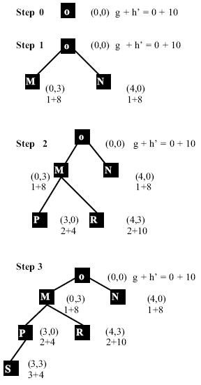
Fig.: Expanding the state-space by the A* algorithm.

Another important issue that needs to be discussed is how to select a path,when an offspring of a currently expanded node is an already existing node. Under this circumstance, the parent that yields a lower value of g+h' for the offspring node is chosen and the other parent is ignored, sometimes by de-linking the corresponding arc from that parent to the offspring node.