Introduction to Neural Networks

Introduction

What is an artificial neural network?

An artificial neural network is a system based on the operation of biological neural networks, in other words, is an emulation of biological neural system. Why would be necessary the implementation of artificial neural networks?
Although computing these days is truly advanced, there are certain tasks that a program made for a common microprocessor is unable to perform; even so a software implementation of a neural network can be made with their advantages and disadvantages.

Advantages:

A neural network can perform tasks that a linear program can not.
When an element of the neural network fails, it can continue without any problem by their parallel nature.
A neural network learns and does not need to be reprogrammed.
It can be implemented in any application.
It can be implemented without any problem.

Disadvantages:

The neural network needs training to operate.
The architecture of a neural network is different from the architecture of microprocessors therefore needs to be emulated.
Requires high processing time for large neural networks.

Another aspect of the artificial neural networks is that there are different architectures, which consequently requires different types of algorithms, but despite to be an apparently complex system, a neural network is relatively simple.

Artificial neural networks are among the newest signal processing technologies nowadays. The field of work is very interdisciplinary, but the explanation I will give you here will be restricted to an engineering perspective.

In the world of engineering, neural networks have two main functions: Pattern classifiers and as non linear adaptive filters. As its biological predecessor, an artificial neural network is an adaptive system. By adaptive, it means that each parameter is changed during its operation and it is deployed for solving the problem in matter. This is called the training phase.

A artificial neural network is developed with a systematic step-by-step procedure which optimizes a criterion commonly known as the learning rule. The input/output training data is fundamental for these networks as it conveys the information which is necessary to discover the optimal operating point. In addition, a non linear nature make neural network processing elements a very flexible system.

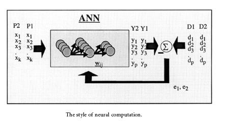
Basically, an artificial neural network is a system. A system is a structure that receives an input, process the data, and provides an output. Commonly, the input consists in a data array which can be anything such as data from an image file, a WAVE sound or any kind of data that can be represented in an array. Once an input is presented to the neural network, and a corresponding desired or target response is set at the output, an error is composed from the difference of the desired response and the real system output.

The error information is fed back to the system which makes all adjustments to their parameters in a systematic fashion (commonly known as the learning rule). This process is repeated until the desired output is acceptable. It is important to notice that the performance hinges heavily on the data. Hence, this is why this data should pre-process with third party algorithms such as DSP algorithms.

In neural network design, the engineer or designer chooses the network topology, the trigger function or performance function, learning rule and the criteria for stopping the training phase. So, it is pretty difficult determining the size and parameters of the network as there is no rule or formula to do it. The best we can do for having success with our design is playing with it. The problem with this method is when the system does not work properly it is hard to refine the solution. Despite this issue, neural networks based solution is very efficient in terms of development, time and resources. By experience, I can tell that artificial neural networks provide real solutions that are difficult to match with other technologies.

Fifteen years ago, Denker said: “artificial neural networks are the second best way to implement a solution” this motivated by their simplicity, design and universality. Nowadays, neural network technologies are emerging as the technology choice for many applications, such as patter recognition, prediction, system identification and control.

The Biological Model

Artificial neural networks born after McCulloc and Pitts introduced a set of simplified neurons in 1943. These neurons were represented as models of biological networks into conceptual components for circuits that could perform computational tasks. The basic model of the artificial neuron is founded upon the functionality of the biological neuron. By definition, “Neurons are basic signaling units of the nervous system of a living being in which each neuron is a discrete cell whose several processes are from its cell body”

biological neural network

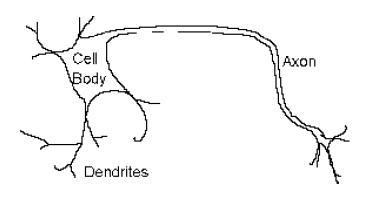
The biological neuron has four main regions to its structure. The cell body, or soma, has two offshoots from it. The dendrites and the axon end in pre-synaptic terminals. The cell body is the heart of the cell. It contains the nucleolus and maintains protein synthesis. A neuron has many dendrites, which look like a tree structure, receives signals from other neurons.

A single neuron usually has one axon, which expands off from a part of the cell body. This I called the axon hillock. The axon main purpose is to conduct electrical signals generated at the axon hillock down its length. These signals are called action potentials.

The other end of the axon may split into several branches, which end in a pre-synaptic terminal. The electrical signals (action potential) that the neurons use to convey the information of the brain are all identical. The brain can determine which type of information is being received based on the path of the signal.

The brain analyzes all patterns of signals sent, and from that information it interprets the type of information received. The myelin is a fatty issue that insulates the axon. The non-insulated parts of the axon area are called Nodes of Ranvier. At these nodes, the signal traveling down the axon is regenerated. This ensures that the signal travel down the axon to be fast and constant.

The synapse is the area of contact between two neurons. They do not physically touch because they are separated by a cleft. The electric signals are sent through chemical interaction. The neuron sending the signal is called pre-synaptic cell and the neuron receiving the electrical signal is called postsynaptic cell.

The electrical signals are generated by the membrane potential which is based on differences in concentration of sodium and potassium ions and outside the cell membrane.

Biological neurons can be classified by their function or by the quantity of processes they carry out. When they are classified by processes, they fall into three categories: Unipolar neurons, bipolar neurons and multipolar neurons.

Unipolar neurons have a single process. Their dendrites and axon are located on the same stem. These neurons are found in invertebrates.

Bipolar neurons have two processes. Their dendrites and axon have two separated processes too.

Multipolar neurons: These are commonly found in mammals. Some examples of these neurons are spinal motor neurons, pyramidal cells and purkinje cells.

When biological neurons are classified by function they fall into three categories. The first group is sensory neurons. These neurons provide all information for perception and motor coordination. The second group provides information to muscles, and glands. There are called motor neurons. The last group, the interneuronal, contains all other neurons and has two subclasses. One group called relay or protection interneurons. They are usually found in the brain and connect different parts of it. The other group called local interneurons are only used in local circuits.

The Mathematical Model

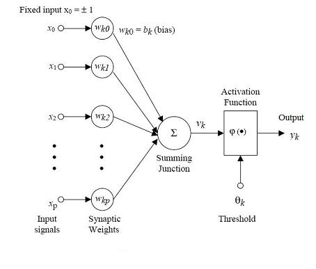
Once modeling an artificial functional model from the biological neuron, we must take into account three basic components. First off, the synapses of the biological neuron are modeled as weights. Let’s remember that the synapse of the biological neuron is the one which interconnects the neural network and gives the strength of the connection. For an artificial neuron, the weight is a number, and represents the synapse. A negative weight reflects an inhibitory connection, while positive values designate excitatory connections. The following components of the model represent the actual activity of the neuron cell. All inputs are summed altogether and modified by the weights. This activity is referred as a linear combination. Finally, an activation function controls the amplitude of the output. For example, an acceptable range of output is usually between 0 and 1, or it could be -1 and 1.

Mathematically, this process is described in the figure

From this model the interval activity of the neuron can be shown to be:

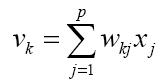
The output of the neuron, yk, would therefore be the outcome of
some activation function on the value of vk.

Activation functions

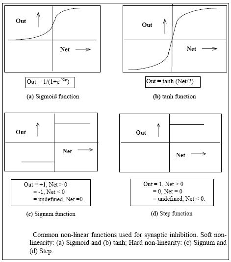
As mentioned previously, the activation function acts as a
squashing function, such that the output of a neuron in a neural network is between
certain values (usually 0 and 1, or -1 and 1). In general, there are
three types of activation functions, denoted by Φ(.) .
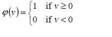
First, there is the Threshold Function which takes on a value of 0 if
the summed input is less than a certain threshold value (v), and the
value 1 if the summed input is greater than or equal to the
threshold value.

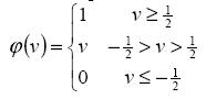
Secondly, there is the Piecewise-Linear function. This function
again can take on the values of 0 or 1, but can also take on values
between that depending on the amplification factor in a certain
region of linear operation.

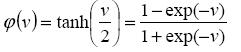
Thirdly, there is the sigmoid function. This function can range
between 0 and 1, but it is also sometimes useful to use the -1 to 1
range. An example of the sigmoid function is the hyperbolic
tangent function.

The artifcial neural networks which we describe are all variations on the parallel
distributed processing (PDP) idea. The architecture of each neural network is based on very similar
building blocks which perform the processing. In this chapter we first discuss these processing
units and discuss diferent neural network topologies. Learning strategies as a basis for an adaptive
system

A framework for distributed representation

An artifcial neural network consists of a pool of simple processing units which communicate by sending
signals to each other over a large number of weighted connections.
A set of major aspects of a parallel distributed model can be distinguished :

a set of processing units (‘neurons,’ ‘cells’);
a state of activation yk for every unit, which equivalent to the output of the unit;
connections between the units. Generally each connection is defined by a weight wjk which
determines the effect which the signal of unit j has on unit k;
a propagation rule, which determines the effective input sk of a unit from its external
inputs;
an activation function Fk, which determines the new level of activation based on the
efective input sk(t) and the current activation yk(t) (i.e., the update);
an external input (aka bias, offset) øk for each unit;
a method for information gathering (the learning rule);
an environment within which the system must operate, providing input signals and|if
necessary|error signals.

Processing units

Each unit performs a relatively simple job: receive input from neighbours or external sources
and use this to compute an output signal which is propagated to other units. Apart from this
processing, a second task is the adjustment of the weights. The system is inherently parallel in
the sense that many units can carry out their computations at the same time.
Within neural systems it is useful to distinguish three types of units: input units (indicated
by an index i) which receive data from outside the neural network, output units (indicated by an index o) which send data out of the neural network, and hidden units (indicated by an index
h) whose input and output signals remain within the neural network.
During operation, units can be updated either synchronously or asynchronously. With synchronous
updating, all units update their activation simultaneously; with asynchronous updating,
each unit has a (usually fixed) probability of updating its activation at a time t, and usually

only one unit will be able to do this at a time. In some cases the latter model has some
advantages.

Neural Network topologies

In the previous section we discussed the properties of the basic processing unit in an artificial
neural network. This section focuses on the pattern of connections between the units and the
propagation of data.
As for this pattern of connections, the main distinction we can make is between:

Feed-forward neural networks, where the data
ow from input to output units is strictly feedforward.
The data processing can extend over multiple (layers of) units, but no feedback
connections are present, that is, connections extending from outputs of units to inputs of
units in the same layer or previous layers.
Recurrent neural networks that do contain feedback connections. Contrary to feed-forward networks,
the dynamical properties of the network are important. In some cases, the activation
values of the units undergo a relaxation process such that the neural network will evolve to
a stable state in which these activations do not change anymore. In other applications,
the change of the activation values of the output neurons are significant, such that the
dynamical behaviour constitutes the output of the neural network (Pearlmutter, 1990).

Classical examples of feed-forward neural networks are the Perceptron and Adaline. Examples of recurrent networks have been presented by Anderson

(Anderson, 1977), Kohonen (Kohonen, 1977), and Hopfield (Hopfield, 1982) .

Training of artifcial neural networks

A neural network has to be configured such that the application of a set of inputs produces
(either ‘direct’ or via a relaxation process) the desired set of outputs. Various methods to set
the strengths of the connections exist. One way is to set the weights explicitly, using a priori
knowledge. Another way is to ‘train’ the neural network by feeding it teaching patterns and
letting it change its weights according to some learning rule.

We can categorise the learning situations in two distinct sorts. These are:

Supervised learning or Associative learning in which the network is trained by providing
it with input and matching output patterns. These input-output pairs can be provided by
an external teacher, or by the system which contains the neural network (self-supervised).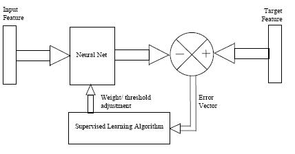
Unsupervised learning or Self-organisation in which an (output) unit is trained to respond
to clusters of pattern within the input. In this paradigm the system is supposed to discover
statistically salient features of the input population. Unlike the supervised learning
paradigm, there is no a priori set of categories into which the patterns are to be classified;
rather the system must develop its own representation of the input stimuli.
Reinforcement Learning This type of learning may be considered as an intermediate form of the above
two types of learning. Here the learning machine does some action on the
environment and gets a feedback response from the environment. The learning
system grades its action good (rewarding) or bad (punishable) based on the
environmental response and accordingly adjusts its parameters.
Generally, parameter adjustment is continued until an equilibrium state occurs,
following which there will be no more changes in its parameters. The selforganizing
neural learning may be categorized under this type of learning.

Modifying patterns of connectivity of Neural Networks

Both learning paradigms supervised learning and unsupervised learning result in an adjustment of the weights of the connections
between units, according to some modification rule. Virtually all learning rules for models
of this type can be considered as a variant of the Hebbian learning rule suggested by Hebb in
his classic book Organization of Behaviour (1949) (Hebb, 1949). The basic idea is that if two
units j and k are active simultaneously, their interconnection must be strengthened. If j receives
input from k, the simplest version of Hebbian learning prescribes to modify the weight wjk with

where ϒ is a positive constant of proportionality representing the learning rate. Another common
rule uses not the actual activation of unit k but the difference between the actual and desired
activation for adjusting the weights:

in which dk is the desired activation provided by a teacher. This is often called the Widrow-Hoff
rule or the delta rule, and will be discussed in the next chapter.
Many variants (often very exotic ones) have been published the last few years.

Neuro AI

Artificial Neural Networks, Algorithms, tutorials and sofware