Genetic Algorithms

Introduction

Professor John Holland in 1975 proposed an attractive class of computational
models, called Genetic Algorithms (GA), that mimic the biological
evolution process for solving problems in a wide domain. The mechanisms
under GA have been analyzed and explained later by Goldberg, De
Jong, Davis, Muehlenbein, Chakraborti, Fogel, Vose
and many others. Genetic Aalgorithms has three major applications, namely, intelligent
search, optimization and machine learning. Currently, Genetic Algorithms is used along with
neural networks and fuzzy logic for solving more complex problems. Because of their joint usage in many problems, these together are often referred to by a
generic name: “;soft-computing”.
A Genetic Algorithms operates through a simple cycle of stages:

i) Creation of a “;population” of strings,
ii) Evaluation of each string,
iii) Selection of best strings and
iv) Genetic manipulation to create new population of strings.

The cycle of a Genetic Algorithms is presented below

Genetic Algorithms Cycle

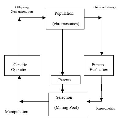
Each cycle in Genetic Algorithms produces a new generation of possible solutions for a
given problem. In the first phase, an initial population, describing
representatives of the potential solution, is created to initiate the search
process. The elements of the population are encoded into bit-strings, called chromosomes. The performance of the strings, often called fitness, is then
evaluated with the help of some functions, representing the constraints of the
problem. Depending on the fitness of the chromosomes, they are selected for a
subsequent genetic manipulation process. It should be noted that the selection
process is mainly responsible for assuring survival of the best-fit individuals.
After selection of the population strings is over, the genetic manipulation
process consisting of two steps is carried out. In the first step, the crossover
operation that recombines the bits (genes) of each two selected strings
(chromosomes) is executed. Various types of crossover operators are found in
the literature. The single point and two points crossover operations are
illustrated
. The crossover points of any two
chromosomes are selected randomly. The second step in the genetic
manipulation process is termed mutation, where the bits at one or more
randomly selected positions of the chromosomes are altered. The mutation
process helps to overcome trapping at local maxima. The offsprings produced
by the genetic manipulation process are the next population to be evaluated.

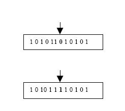
Fig.: Mutation of a chromosome at the 5th bit position.

Example: The Genetic Algorithms cycle is illustrated in this example for maximizing a
function f(x) = x2 in the interval 0 = x = 31. In this example the fitness
function is f (x) itself. The larger is the functional value, the better is the
fitness of the string. In this example, we start with 4 initial strings. The fitness
value of the strings and the percentage fitness of the total are estimated in
Table A. Since fitness of the second string is large, we select 2 copies of the
second string and one each for the first and fourth string in the mating pool.
The selection of the partners in the mating pool is also done randomly. Here in
table B, we selected partner of string 1 to be the 2-nd string and partner of
4-th string to be the 2nd string. The crossover points for the first-second and
second-fourth strings have been selected after o-th and 2-nd bit positions
respectively in table B. The second generation of the population without
mutation in the first generation is presented in table C.
Table A:

Table B: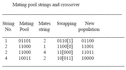

Table C: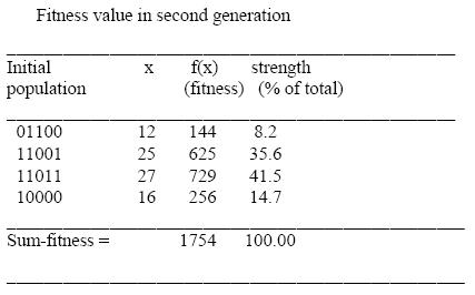

A Schema (or schemata in plural form) / hyperplane or similarity
template is a genetic pattern with fixed values of 1 or 0 at some
designated bit positions. For example, S = 01?1??1 is a 7-bit schema with
fixed values at 4-bits and don’t care values, represented by ?, at the remaining
3 positions. Since 4 positions matter for this schema, we say that the schema
contains 4 genes.

Deterministic Explanation of
Holland’s Observation

To explain Holland’s observation in a deterministic manner let us presume the following assumptions.

i) There are no recombination or alternations to genes.

ii) Initially, a fraction f of the population possesses the schema S and those
individuals reproduce at a fixed rate r.

iii) All other individuals lacking schema S reproduce at a rate s < r.

Thus with an initial population size of N, after t generations, we find Nf r t
individuals possessing schema S and the population of the rest of the
individuals is N(1 - f) st. Therefore, the fraction of the individuals with
schema S is given by

For small t and f, the above fraction reduces to f (r / s) t , which
means the population having the schema S increases exponentially at a rate
(r / s). A stochastic proof of the above property will be presented shortly, vide
a well-known theorem, called the fundamental theorem of Genetic
algorithm.

Stochastic Explanation of Genetic Algorithms

For presentation of the fundamental theorem of Genetic Algorithms, the following
terminologies are defined in order.

Definition: The order of a schema H, denoted by O(H), is the number
of fixed positions in the schema. For example, the order of schema H =
?001?1? is 4, since it contains 4 fixed positions.

For example, the schema ?1?001 has a defining length d(H) = 4 - 0 = 4, while
the d(H) of ???1?? is zero.

Definition: The schemas defined over L-bit strings may be
geometrically interpreted as hyperplanes in an L- dimensional hyperspace
(a binary vector space) with each L-bit string representing one corner point in
an n-dimensional cube.

The Fundamental Theorem of Genetic Algorithms

(Schema theorem)

Let the population size be N, which contains mH (t) samples of schema H at
generation t. Among the selection strategies, the most common is the
proportional selection. In proportional selection, the number of copies of
chromosomes selected for mating is proportional to their respective fitness
values. Thus, following the principles of proportional selection, a string i
is selected with probability

where fi is the fitness of string i. Now, the probability that in a single
selection a sample of schema H is chosen is described by

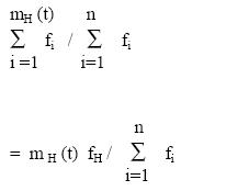
where f H is the average fitness of the mH (t) samples of H.

Thus, in a total of N selections with replacement, the expected number of
samples of schema H in the next generation is given by

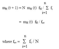
where fav is the population average fitness in generation t. The last expression
describes that the Genetic algorithm allocates over an increasing number of
trials to an above average schema. The effect of crossover and mutation can be
incorporated into the analysis by computing the schema survival probabilities
of the above average schema. In crossover operation, a schema H survives if
the cross-site falls outside the defining length d(H). If pc is the probability of
crossover and L is the word-length of the chromosomes, then the disruption
probability of schema H due to crossover is

A schema H, on the other hand, survives mutation, when none of its
fixed positions is mutated. If pm is the probability of mutation and O(H) is the
order of schema H, then the probability that the schema survives is given by

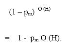
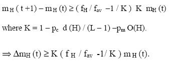
Therefore, under selection, crossover and mutation, the sample size of
schema H in generation (t + 1) is given by

The above theorem is called the fundamental theorem of GA or the
Schema theorem. It is evident from the Schema theorem that for a given set
of values of d(H), O(H), L, pc and pm , the population of schema H at the
subsequent generations increases exponentially when fH > fav. This, in fact,
directly follows from the difference equation:

Replacing Δ by (E -1), where E is the extended difference operator, we find

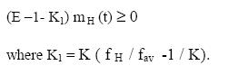
Since m H (t) in equation (E-1-K1)mH(t) ≥ 0 is positive, E ≥ (1 +K1 ). Thus, the
solution of (15.12) is given by

where A is a constant. Setting the boundary condition at t = 0, and substituting
the value of K1 by therein, we finally have:

Since K is a positive number, and f H / fav > 1, mH (t) grows
exponentially with iterations. The process of exponential increase of mH (t)
continues until some iteration r, when fH approaches fav. This is all about the
proof of the schema theorem.

The Markov Model for
Convergence Analysis

For the sake of understanding, let us now consider the population size =
3 and the chromosomes are 2-bit patterns, as presumed earlier. The set S now
takes the following form.

S = {(00, 00, 00), (00, 00, 01), (00, 00, 10), (00, 00, 11),
(00, 01, 00), (00, 01, 01), (00, 01, 10), (00, 01, 11),
…. … ….. …..
…. … …. ….
(11, 11, 00), (11, 11, 01), (11, 11, 10), (11, 11, 11) }

It may be noted that the number of elements of the last set S is 64. In
general, if the chromosomes have the word length of m bits and the number of
chromosomes selected in each Genetic Algorithm cycle is n, then the cardinality of the set S
is 2 ^ mn.
The Markov transition probability matrix P for 2-bit strings of
population size 2, thus, will have a dimension of (16 x 16), where the element
pij of the matrix denotes the probability of transition from i-th to j-th state. A
clear idea about the states and their transitions can be formed from fig.

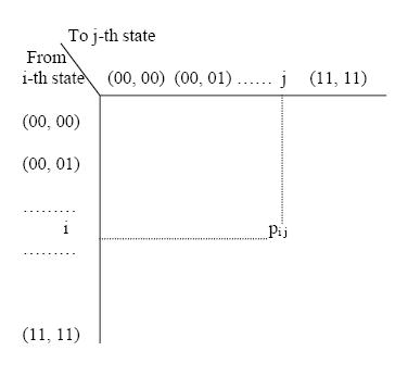
It needs mention that since from a given i-th state, there could be a
transition to any 16 j-th states, therefore the row sum of P matrix must be 1.
Formally,

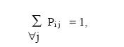
for a given i.

Now, let us assume a row vector πt, whose k-th element denotes the
probability of occurrence of the k-th state at a given genetic iteration (cycle) t;
then πt + 1 can be evaluated by

Thus starting with a given initial row vector π0 , one can evaluate the state
probability vector after n-th iteration πn by

The behavior of Genetic Algorihms without mutation can be of the following three types.

i) The GA may converge to one or more absorbing states (i.e., states
wherefrom the GA has no transitions to other states).
ii) The GA may have transition to some states, wherefrom it may
terminate to one or more absorbing states.
iii) The GA never reaches an absorbing state.

Taking all the above into account, we thus construct P as a partitioned matrix
of the following form:

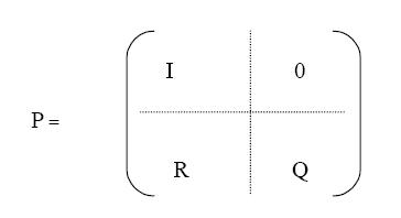
where I is an identity matrix of dimension (a x a) that corresponds to the
absorbing states; R is a (t x a) transition sub-matrix describing transition to an
absorbing state; Q is a (t x t) transition sub-matrix describing transition to
transient states and not to an absorbing state and 0 is a null matrix of
dimension (t x t).

It can be easily shown that Pn for the above matrix P can be found to
be as follows.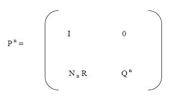

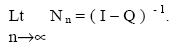
where the n-step transition matrix Nn is given by

As n approaches infinity,

Consequently, as n approaches infinity,

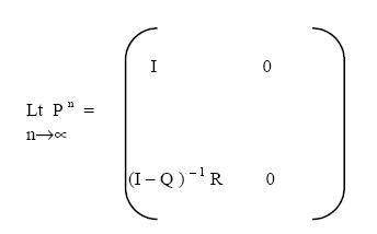
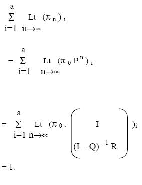
Goodman has shown [8] that the matrix (I - Q) -1 is guaranteed to exist.
Thus given an initial probability vector p 0, the chain will have a transition to
an absorbing state with probability 1. Further, there exists a non-zero
probability that ab sorbing state will be the globally optimal state .
We now explain: why the chain will finally terminate to an absorbing
state. Since the first ‘a’ columns for the matrix Pn, for n→∞, are non-zero and
the remaining columns are zero, therefore, the chain must have transition to
one of the absorbing states. Further, note that the first ‘a’ columns of the row
vector p n for n→∞ denote the probability of absorption at different states,
and the rest of the columns denote that the probability of transition to nonabsorbing
states is zero. Thus probability of transition to absorbing states is
one. Formally,